Subsurface Control of Active-Site Distributions in Pt-Skin HEA Electrocatalysts
From single active sites to engineered active-site populations — tuning H adsorption through the buried composition
H*
Pt skin
HEA subsurface
PtFeCoNiCu
Chen-Cheng Liao (廖振成) Department of Chemistry, Fu Jen Catholic University, New Taipei City, Taiwan DFT & machine learning · 165804@mail.fju.edu.tw
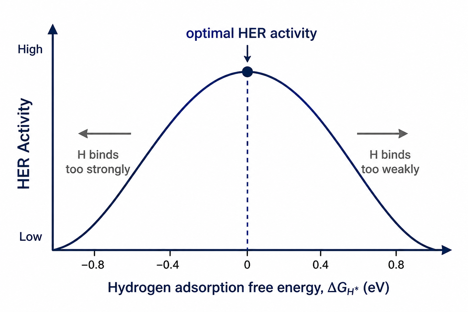
Platinum is the HER benchmark — but it is expensive
HER activity peaks when hydrogen binds at ΔGH* ≈ 0 — right where Pt sits. But Pt is costly and scarce, so the search for cheaper, tunable catalysts continues.
Key messageThe goal: reach Pt-like H binding (ΔGH* ≈ 0) with far less Pt.
Five-plus near-equiatomic elements, randomly mixed — so no two surface sites see the same neighbourhood
Why we care random mixing means every surface site sees a different local environment — one material, a continuum of distinct binding sites.
Five-plus principal elements, each near-equiatomic — a vast, tunable composition space.
High mixing entropy keeps it a single disordered solid solution.
Key messageWhat makes HEAs special for catalysis is local-environment diversity — many distinct sites in one material.
Pt-skin HEA: keep Pt’s surface, tune the buried core
A pure-Pt outer layer over a mixed Fe–Co–Ni–Cu–Pt core — Pt-like chemistry on top, far less Pt and new tunability underneath
The Pt skin preserves Pt-like surface chemistry, while the buried high-entropy environment is used to tune H adsorption.
Key messageKeep a Pt-like surface, let buried atoms tune it, and use less Pt.
HEA catalysis is not a single-site problem
Even under a pure-Pt skin, each hollow sits above a different subsurface — so adsorption becomes a distribution
a few discrete sites
→
a distribution of ΔGH*
→
engineer the active-site population
Key messageActivity is a distribution of sites — so the design target is the active-site population, not one site.
Pt-skin: a controlled platform for the buried effect
The adsorbate always meets a Pt-rich surface; the variation comes from the composition underneath
The Pt skin fixes the surface chemistry, while the buried Fe–Co–Ni–Cu–Pt environment tunes the local H adsorption energy.
Key messageThe Pt skin isolates one clean question: how does the buried environment tune surface Pt?
The central question of this work
Can the buried composition set — and let us predict — each site’s H binding, and thus the whole active-site population?
1
Pt-skin slab
SQS surface model
→
2
Hollow-site DFT
per-site ΔGH*
→
3
Local descriptors
subsurface counts
→
4
Adsorption predictor
from local descriptors
→
5
Active-site population
μ, σ, Popt
The buried environment sets each site’s ΔGH*; the target is the resulting active-site population — with DFT as calibration, not a full census, kinetics, or MLP.
Key messageThe target is the active-site population; prediction is the route, and DFT is the calibration.
06
Methods overview
Fe–Co–Ni–Cu–Pt Pt-skin (111): from random structure to descriptors
1
SQS bulk
random alloy in a finite cell
2
Pt-skin slab
4×4×6 · 96 atoms · pure-Pt top
3
96 hollow sites
all FCC + HCP, 3 slabs
4
DFT ΔGH*
VASP, per site
5
Descriptors
local environment · d-band · surrogate prediction
DFT settings
VASP · GGA-PBE 520 eV · spin-polarized Γ-centered 3×3×1
Free energy
ΔGH* = ΔEads + 0.24 eV
computational hydrogen electrode
SQS gives finite periodic slabs whose local statistics approximate a random alloy.
Key messageA controlled 96-site hollow-site dataset across three Pt-skin HEA surfaces.
06 / 18
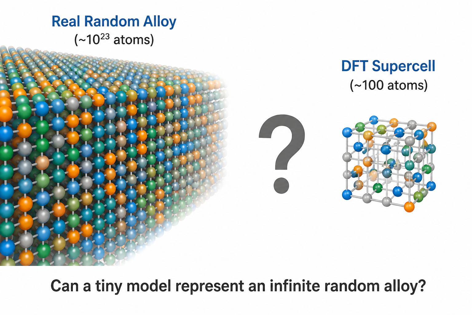
Can a small cell represent an infinite random alloy?
A real random alloy has ~1023 atoms; DFT can treat only ~100 — this is the gap an SQS bridges
A real random alloy is effectively infinite, but DFT can only treat ~100 atoms — the SQS is the small cell built to stand in for it.
Key messageAn SQS lets a ~100-atom DFT cell represent an effectively infinite random alloy.
What is a special quasirandom structure (SQS)?
A small periodic cell built to imitate an infinite random alloy
An SQS reproduces the local atomic statistics of a random alloy — in a cell small enough for DFT.
1
The problem
A real random alloy is effectively infinite — it cannot enter a DFT calculation directly.
→
2
The constraint
DFT needs a finite, periodic cell — whatever it contains repeats forever.
→
3
The trick
Choose the arrangement whose neighbour statistics match a random alloy.
Key messageAn SQS is statistically random — not merely random-looking.
Our model: a Pt-skin (111) high-entropy slab
Top view and side view of the 4×4×6 slab — 96 atoms, six layers
Pt skin on top · Fe–Co–Ni–Cu–Pt below (top 3 relaxed, bottom 3 fixed)
Key messageA pure-Pt skin over the HEA subsurface — the surface looks like Pt; the layers beneath do the tuning.
What we count: the 6 atoms beneath a hollow site
An x-ray view from the Pt skin into the subsurface ring
An H atom adsorbs in a 3-fold hollow site on the Pt skin.
Make the skin transparent: directly beneath sit 6 subsurface atoms — the local ring.
Descriptorls_X = counts in that ring → here Pt 2 · Fe 1 · Co 1 · Ni 1 · Cu 1.
Key messageEach site's descriptor is the element makeup of the 6 atoms under its hollow.
07
The site population sits on the Sabatier optimum
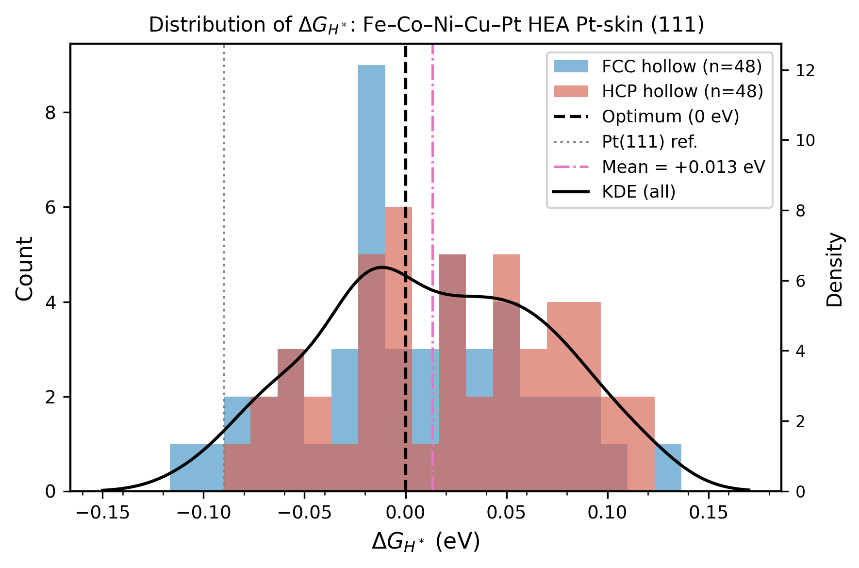
ΔGH* across all 96 sites — tight and near-thermoneutral
Figure 1. ΔGH* distribution over 96 FCC + HCP hollow sites (3 SQS slabs); Pt(111) reference −0.09 eV.
92 %
of sites are already within |ΔGH*| ≤ 0.10 eV — most of the population is near-optimal
+0.013 eV
mean ΔGH* — essentially thermoneutral
0.055 eV
standard deviation — a narrow spread
Key messageThe Pt-skin HEA naturally creates a near-optimal population of H-binding sites.
07 / 18
Local descriptors are compositionally constrained
Each hollow site samples six subsurface atoms, so increasing one element necessarily decreases others
lsPt + lsNi + lsCo + lsFe + lsCu = 6
Each site is described by the six subsurface atoms beneath it. Because the five elemental counts always sum to six, the descriptors are not independent.
Caution Raw correlations are useful, but they mix chemical trends with compositional coupling.
Key messageBecause the five counts sum to six, raw correlations are useful for screening — not for independent elemental interpretation.
Raw Pearson: apparent Pt-rich and Fe-rich trends
Pt-rich environments bind H more strongly; Fe-rich environments bind H more weakly
Raw r of each subsurface count vs ΔGH* (n = 96)
ls_Pt−0.64
ls_Fe+0.54
ls_Cu−0.22
ls_Co+0.20
ls_Ni+0.02
Bars left of centre = stronger H binding · right = weaker.
Pt is negatively correlated: more Pt in the local ring → more negative ΔGH* → stronger H binding.
Fe is positively correlated: more Fe in the local ring → more positive ΔGH* → weaker H binding.
CautionApparent ranking — needs a compositional check (counts are closed, so this is not yet an independent Fe effect).
Key messagePt-rich → stronger binding, Fe-rich → weaker — but this is an apparent ranking that still needs a compositional check.
Is Fe only the complement of Pt?
If the five counts sum to six, Fe-rich could simply mean Pt-poor — so we check
Are Fe-rich sites just Pt-poor sites?
+0.54 r
raw correlation of ls_Fe with ΔGH* (weaker-binding side)
Check 1Pt–Fe is not the strongest anti-pair. corr(Pt,Fe) = −0.21, weaker than corr(Pt,Ni) = −0.35 — Fe varies largely independently of Pt.
Check 2Fe stays positive at fixed Pt. Within matched Pt-count groups, r(ls_Fe, ΔGH*) = +0.60 / +0.55 / +0.41 (ls_Pt = 0 / 1 / 2).
Fe is not simply the inverse of Pt. Fe-rich subsurface environments are meaningful weak-binding-side descriptors.
Key messageFe is not just the complement of Pt — it behaves as a meaningful weak-binding-side subsurface descriptor.
Replacement effects give a chemistry-readable ordering
Instead of an absolute effect per element, ask what happens when one subsurface atom is replaced by another
Binding-strength ordering Pt > Cu > Ni > Co > Fe
Fe → Pt replacement: ΔΔGH* ≈ −61 meV — replacing a subsurface Fe by Pt makes H binding stronger. This contrast is reference-invariant under the closed counts.
The ordering broadly tracks Pauling electronegativity, but with only five elements we treat it as chemical consistency, not a statistical proof, and within this dataset.
Key messageReplacement-effect ordering Pt > Cu > Ni > Co > Fe within this dataset — consistent with electronegativity, interpreted as chemical intuition.
11
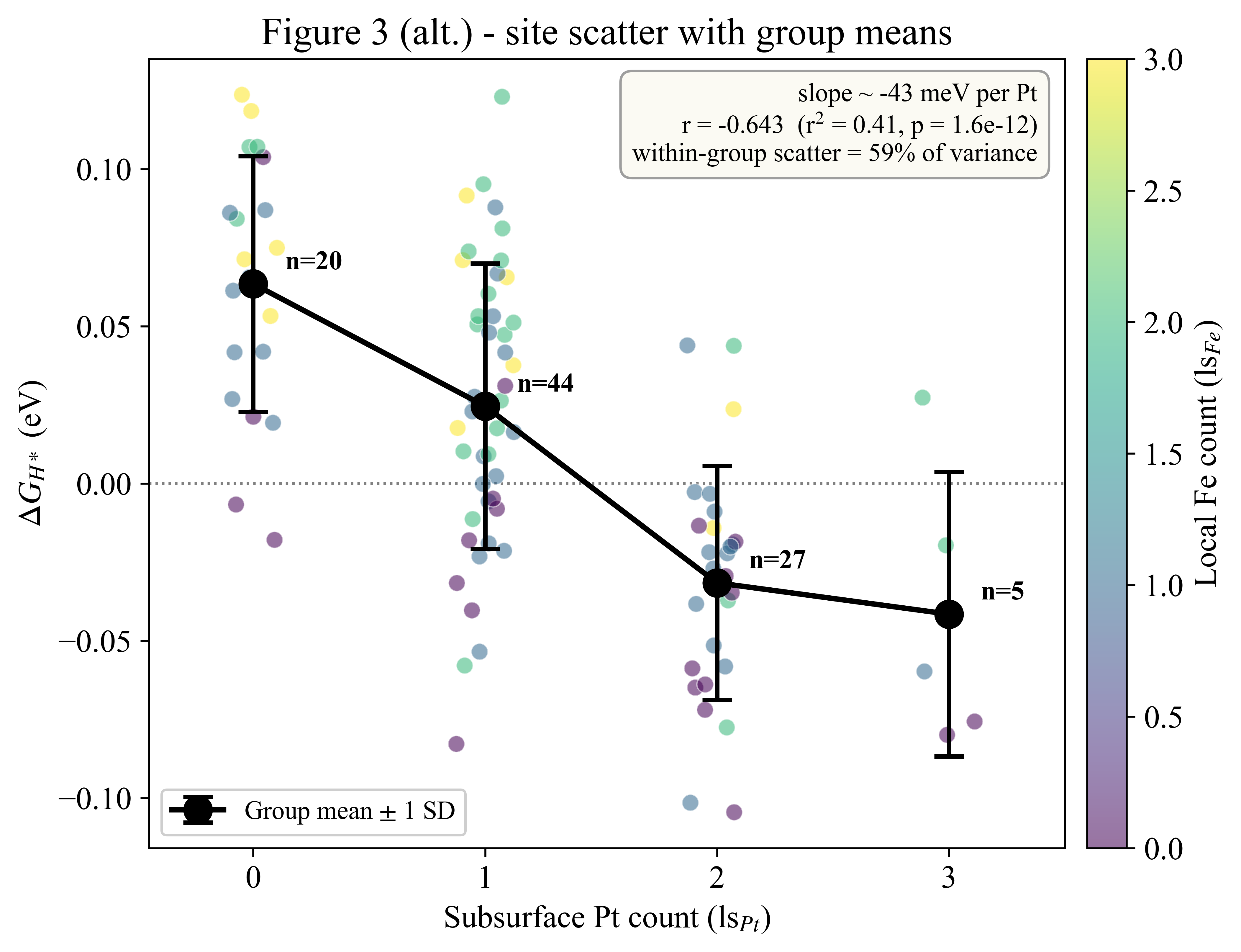
Subsurface Pt is the dominant handle
More Pt beneath the skin → weaker H binding, ΔGH* rising through zero
Figure 3. ΔGH* vs subsurface Pt count; points coloured by local Fe count, black = group mean ± 1 SD. Trend r = −0.64 (≈ −43 meV per subsurface Pt).
−0.64 r
monotonic trend in subsurface Pt count
0 → 3 subsurface Pt walks a site's ΔGH* from positive toward and past the optimum.
Sign convention: higher ΔGH* = weaker H binding.
Key messageOne countable quantity — subsurface Pt — predicts which way H binding moves.
11 / 18
12
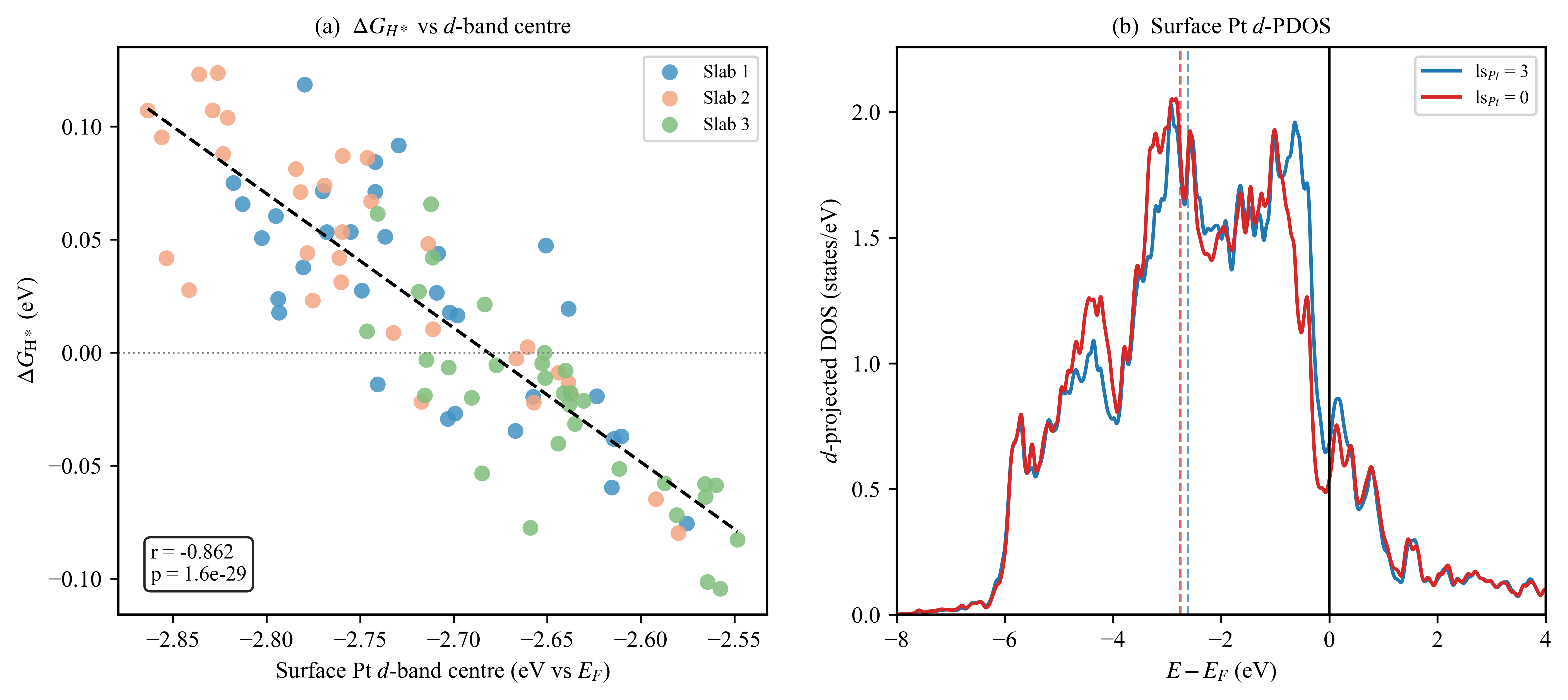
The electronics confirm the mechanism
A site-projected d-band-center effect, measured atom by atom
Figure 6. (a) ΔGH* vs surface-Pt d-band center (r = −0.86). (b) d-projected DOS for high vs low subsurface Pt.
We stop optimizing one site and start engineering the population; the d-band center is the transferable bridge.
Key messageMove from optimizing a single active site to engineering the active-site population — buried composition is the handle.
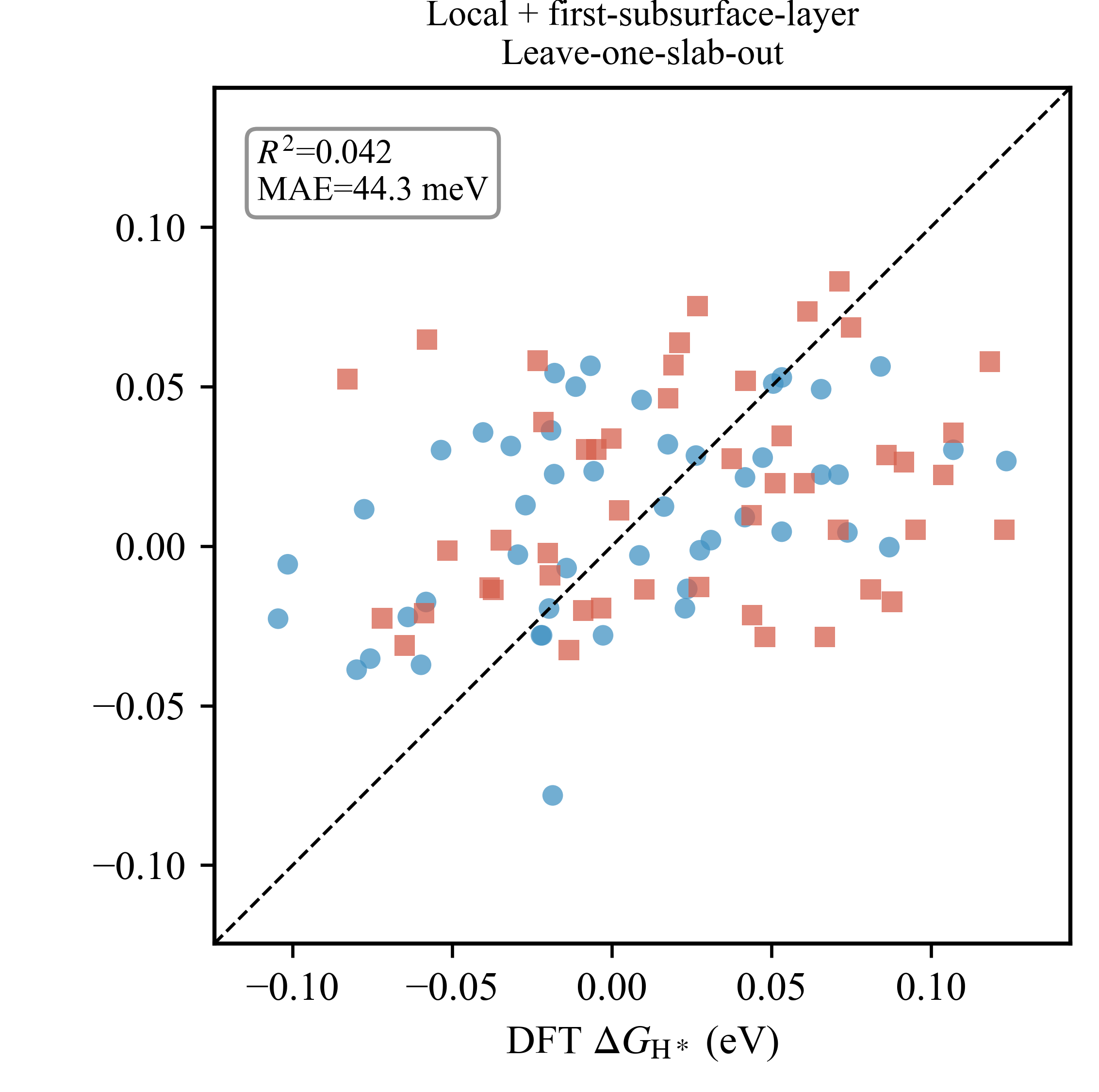
15 / 18
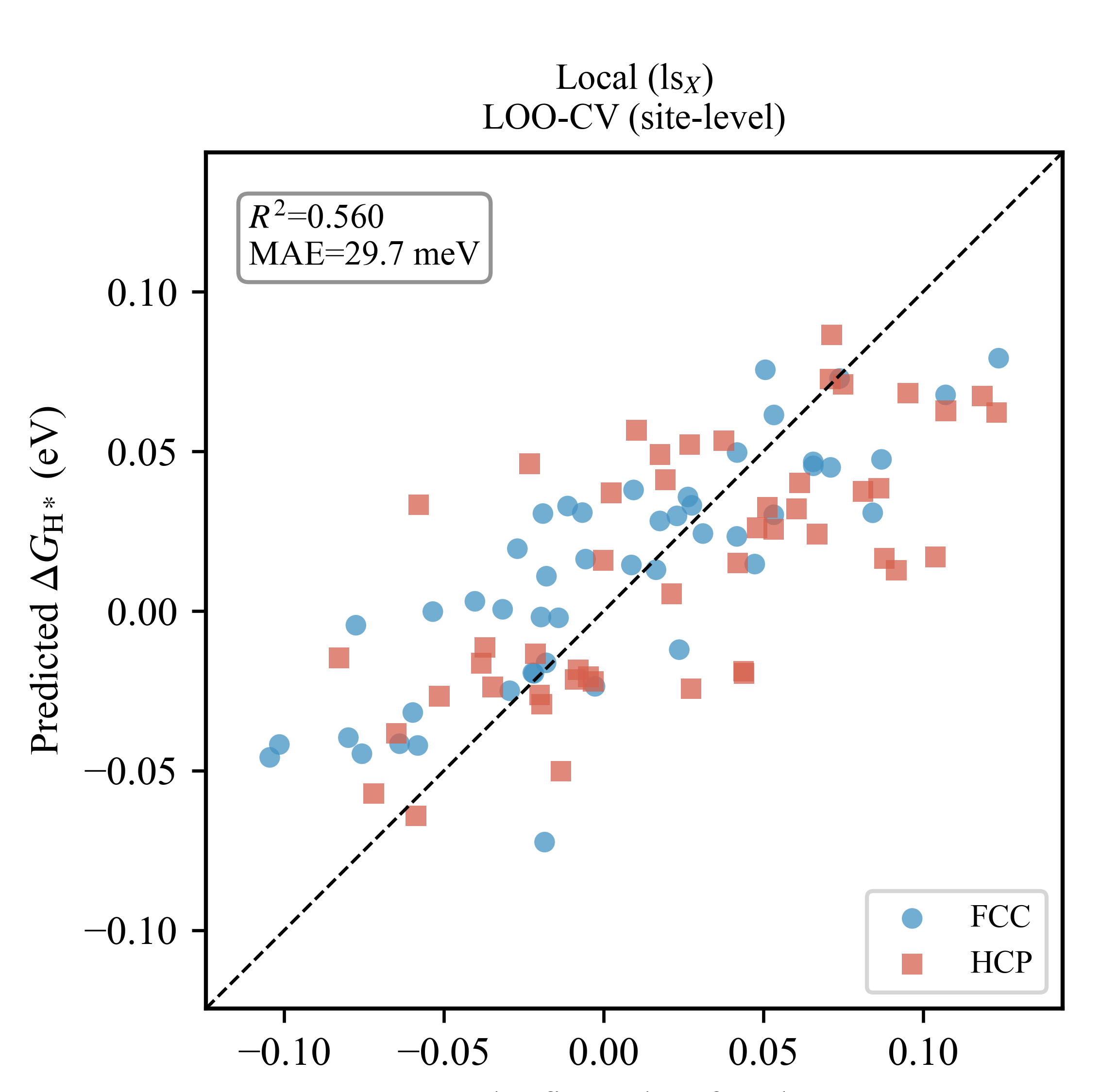
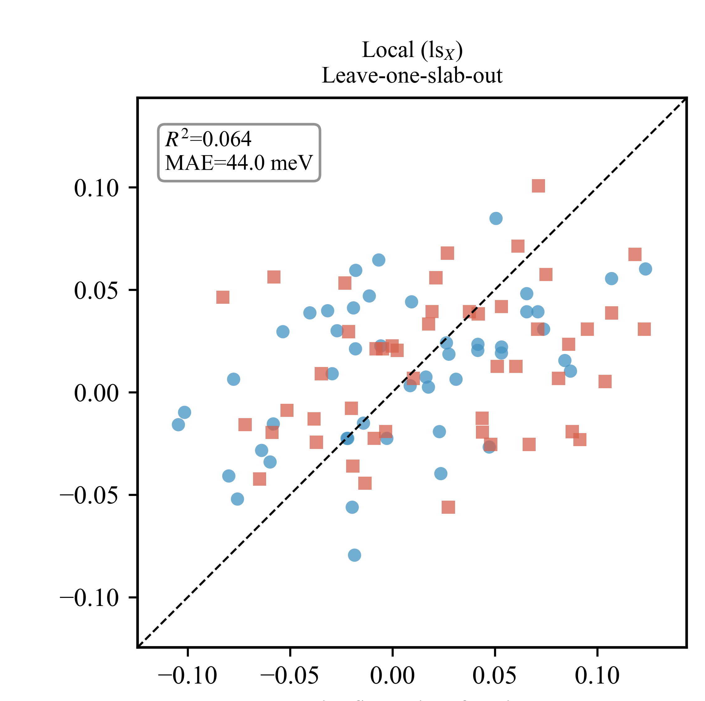
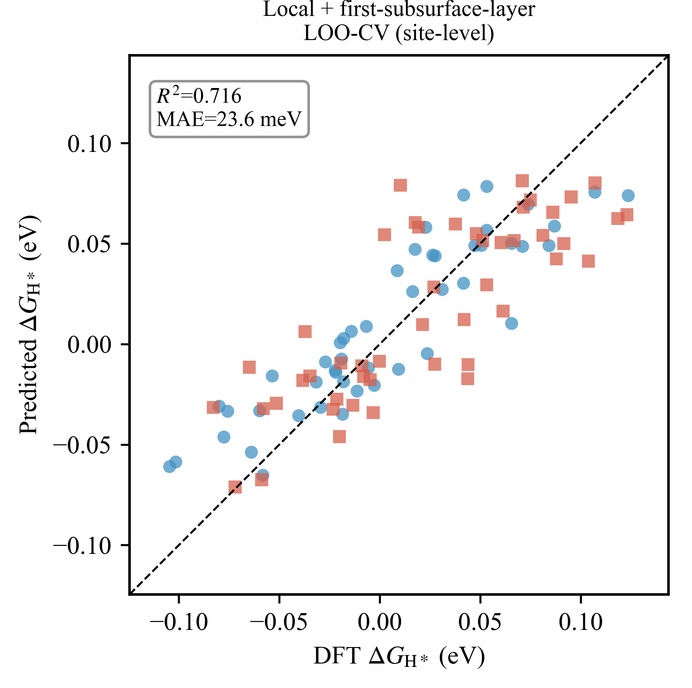
Key messageML defines the scope: local descriptors interpret ΔGH* within sampled slabs (≈ 24–30 meV, site-level) — not extrapolation to unseen compositions.
14 / 18
17
Conclusion
Subsurface control of active-site distributions in Pt-skin HEA
1
HEA catalysis is a population problem
96 Pt-skin hollow sites form a distribution of ΔGH* values — design the population, not one site.
2
Subsurface composition controls H adsorption through the d-band
Within this dataset, subsurface composition modulates the Pt d-band and rationalizes H-binding variations.
3
A starting point for descriptor-guided population design
ML validation limits the claim to within-sampled-slab interpretation; broader design requires more slabs and compositions.
Key messageHEA site heterogeneity is, at heart, a subsurface problem — and, within this dataset, a readable one.
17 / 18
Thank you
Questions welcome
Chen-Cheng Liao (廖振成) · Department of Chemistry, Fu Jen Catholic University 165804@mail.fju.edu.tw · Supported by NSTC 114-2113-M-030-015-MY2 With students Peggy P. M. J. and Yu-Huan Huang (黃宇桓)
Backup · for Q&A
Backup — how the SQS is constructed
Supporting detail for Q&A: choosing the arrangement, and the Monte-Carlo annealing that finds it.
Choosing an SQS: match the neighbours
Same composition, different arrangement — pick the one closest to random
clustered
mismatch: high
partly ordered
medium
random-like
low ✓ SQS
Count each atom's neighbours: the fractions should match the bulk composition.
Minimise the mismatch — the Warren–Cowley parameter α → 0 — over the nearest shells.
Next the following two slides show how that arrangement is actually found.
Key messageThe SQS is chosen by neighbour statistics, not by eye.
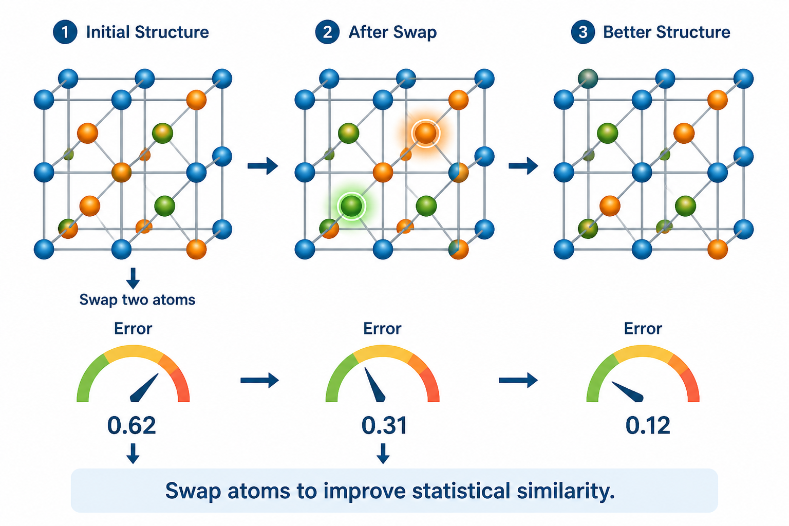
Finding an SQS is an optimization
Swap two atoms, re-score the neighbour statistics, keep what gets closer to random
Each swap proposes a candidate structure; the correlation mismatch (error) falls as the arrangement approaches a random alloy.
Key messageAn SQS is found by minimising the mismatch between its neighbour statistics and a true random alloy.
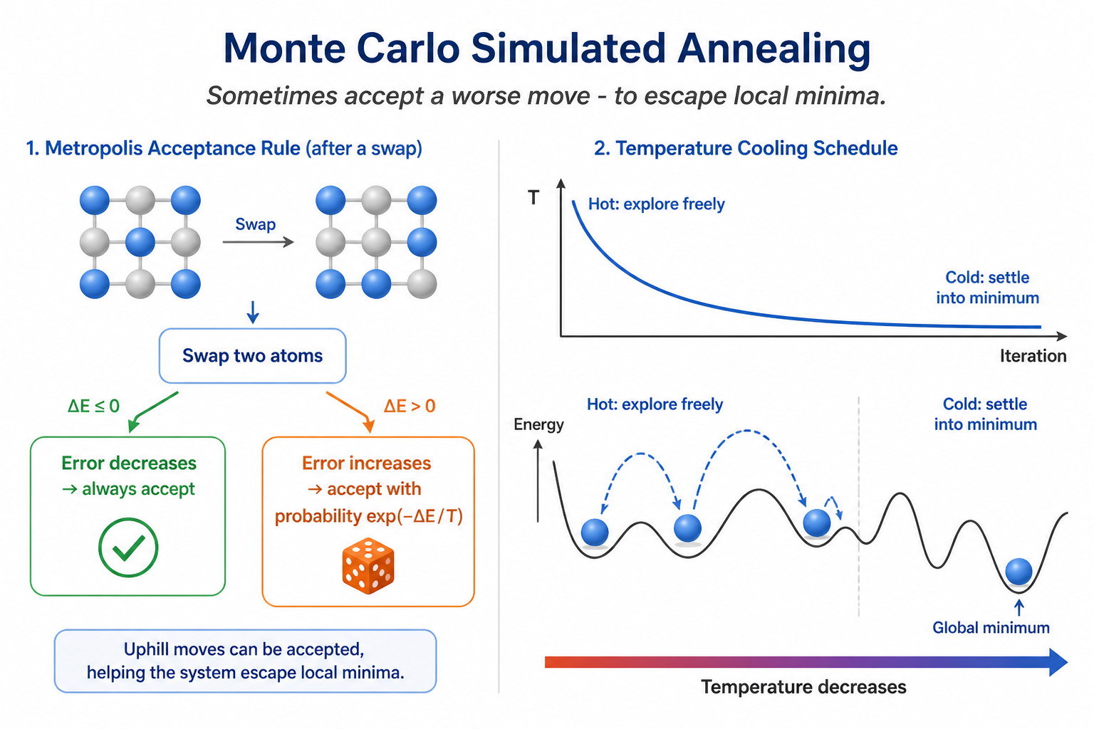
Monte Carlo annealing finds the global best
Always accept improving swaps; accept worsening ones with probability exp(−ΔE/T), cooling slowly
Simulated annealing accepts occasional uphill moves and lowers the "temperature" gradually, so the search escapes local minima and converges to the smallest statistical error.
Key messageAnnealing reaches the SQS with the lowest correlation mismatch — not just a nearby local minimum.
1 / 18
→ / Space reveal & next · ← back · O overview · F fullscreen · P→PDF · (mobile: tap / swipe)